- Entry
- 025
- Source scale
- 0.5 m grid
- Method
- Airborne laser, classified returns
- Section
- Canopy
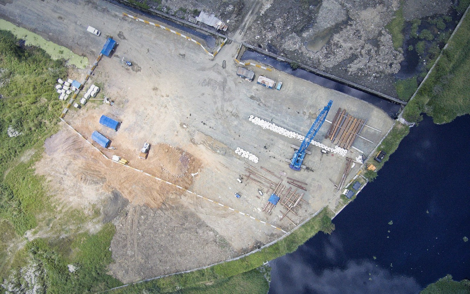
A half-metre grid records more than a sheet can show, and the drawing spacing still has to be chosen afterwards.
Photo: Ferdie Cayanga / PexelsWhat fits in fifty centimetres
When a lidar-derived terrain model is gridded at half-metre resolution, each cell represents a ground patch roughly the size of a paving slab. At that scale, individual plough ridges — typically 30 to 60 centimetres from crest to trough — become legible as distinct rows of alternating high and low returns. Ridge-and-furrow earthworks that vanish completely at the two-metre resolution common in national archive products reappear as unmistakable corrugation. The difference is not cosmetic; it changes what can be measured and what can be missed.
National mapping agencies that operate at this resolution tend to acquire their data at point densities of four returns per square metre or higher — the minimum needed to produce a reliable half-metre bare-earth surface under vegetation. Below that density, the grid interpolates rather than records, and the interpolation can smear exactly the kind of sharp edge a furrow provides.
A surface has to be cut at some spacing before it can be drawn, and the spacing is chosen rather than measured.
Photo: kdadan97 / PexelsThe storage consequence is direct and not trivial. A half-metre grid covers four times the cells of a one-metre grid over the same area, and sixteen times those of a two-metre grid. A single one-kilometre tile in 32-bit floating-point raster format runs to around sixteen megabytes. A national coverage at that resolution — across a country the size of England — sits in the low terabytes, manageable by modern infrastructure but not negligible when every derivative product (slope, aspect, hillshade, curvature) requires its own layer at the same grain.
Tiling conventions matter here more than they do at coarser resolutions. A query that crosses a tile boundary must stitch two or more files, and if the tiles were not classified consistently, a seam can run across a field as a thin discontinuity in elevation values — invisible on a hillshade but measurable in a profile.

Field and desk are separate operations, reconciled only where control has been established.
For anyone using half-metre data seriously, the practical question is not whether the resolution is high enough. It almost always is. The question is whether the acquisition density, the classification parameters, and the tiling scheme were applied consistently enough for the detail the grid appears to offer to be real.