- Entry
- 026
- Source scale
- 0.5 m grid
- Method
- Airborne laser, classified returns
- Section
- Canopy
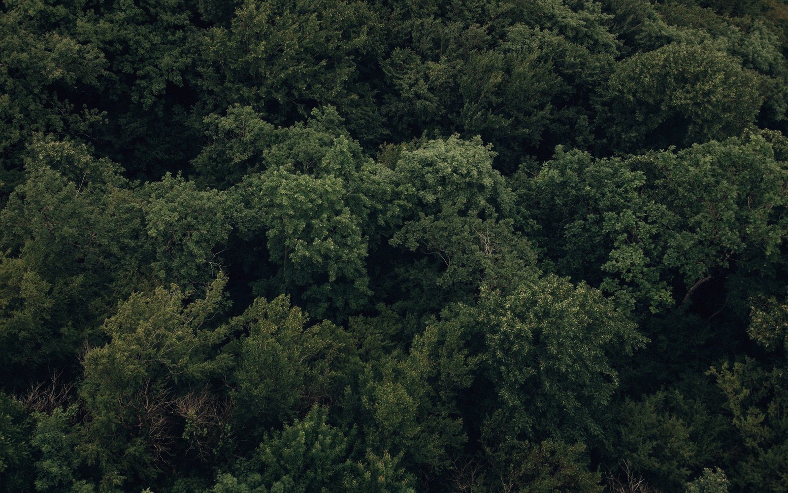
Steep ground facing away from the flight line is sampled least, and the model is quietest exactly where it is least certain.
Photo: ROMAN ODINTSOV / PexelsThe gaps a classifier cannot fill
Airborne LiDAR works by timing the return of laser pulses fired at the ground. Under deciduous woodland in winter, gaps in the canopy are wide enough that some fraction of each pulse reaches bare earth and bounces back. The classifier reads the late-arriving return as ground, and the bare-earth model emerges. Dense evergreen canopy — mature Norway spruce, Sitka plantation, old Scots pine — changes that geometry. The needles intercept pulses at every level, scattering energy before it reaches the forest floor. Returns cluster in the upper and mid canopy; the last return that the classifier promotes to "ground" is often still a metre or more above the soil. The resulting digital terrain model is systematically too high, and the error is not random — it follows the stand boundaries exactly.
Standing water is a different failure mode. A flat water surface at the right angle of incidence reflects the pulse away from the sensor like a mirror. The detector receives nothing back, or receives a faint, ambiguous return from turbidity or surface ripple. The processing software interpolates across the gap using neighbouring points. What fills in is whatever the algorithm assumes — usually a flat continuation of the surrounding terrain. If that terrain slopes toward the water, the interpolated surface may be meaningless, and a shallow wetland can vanish entirely from the bare-earth model, replaced by a smooth plain that was never there.

Every sheet crosses a table like this one before it is printed, and picks up a decision at each pass.
Steep ground facing away from the flight line is the third condition, and it compounds the others. LiDAR surveys are flown along parallel swaths, each offset from the last, with enough overlap to give most surfaces adequate point density. A slope angled away from the sensor presents a narrow cross-section to the incoming pulses. Point density drops sharply — sometimes to a single return per square metre on gradients above thirty degrees. Gullies and north-facing scarps that run oblique to the flight lines can come back nearly empty. The standard fix is to fly crossing flight lines, but this doubles survey time and cost, and many operational surveys — particularly older ones from the first decade of routine LiDAR acquisition — did not do it.
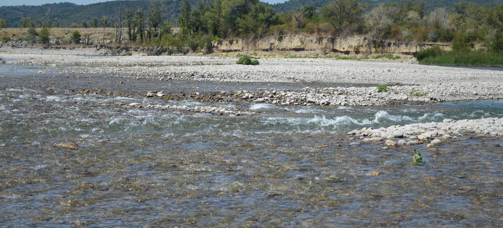
At low flow the channel occupies a fraction of its bed. The edge drawn on a sheet belongs to the day it was surveyed.
Photo: SlimMars 13 / PexelsThe practical consequence for anyone reading a bare-earth model: check the metadata for flight-line direction and season of acquisition before trusting contours under conifers, along stream margins, or across ground with significant relief. The model looks authoritative; the point cloud it was built from may have left whole patches to inference.
- Dense evergreen canopylast returns stay above soil level; bare-earth model reads systematically high
- Standing waterspecular reflection loses the pulse; processor interpolates, often incorrectly
- Steep ground away from flight linepoint density collapses; gullies and scarps may be nearly empty